Basic Example
This example is a basic introduction to using pydftools. It mimics
example 1 of dftools.
In [1]:
# Import relevant libraries
%matplotlib inline

import pydftools as df
import time

 # Make figures a little bigger in the notebook
import matplotlib as mpl
mpl.rcParams['figure.dpi'] = 120

# For displaying equations
from IPython.display import display, Markdown
Choose some parameters to use throughout
In [2]:
n = 1000
seed = 1234
sigma = 0.5
model =df.model.Schechter()
p_true = model.p0
Generate mock data with observing errors:
In [3]:
data, selection, model, other = df.mockdata(n = n, seed = seed, sigma = sigma, model=model, verbose=True)
Number of sources in the mock survey (expected): 1000.000
Number of sources in the mock survey (selected): 1000
Create a fitting object (the fit is not performed until the fit
object is accessed):
In [4]:
survey = df.DFFit(data=data, selection=selection, model=model)
Perform the fit and get the best set of parameters:
In [5]:
start = time.time()
print(survey.fit.p_best)
print("Time for fitting: ", time.time() - start, " seconds")
[ -2.04370588  11.12540248  -1.29867552]
Time for fitting:  0.47102880477905273  seconds
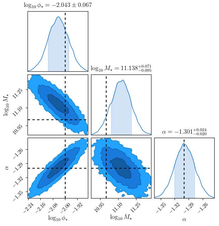
Plot the covariances:
In [6]:
fig = df.plotting.plotcov([survey], p_true=p_true, figsize=1.3)
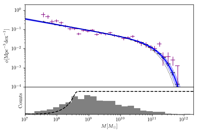
Plot the mass function itself:
In [7]:
fig, ax = df.mfplot(survey, xlim=(1e7,2e12), ylim=(1e-4,2), p_true = p_true, bin_xmin=7.5, bin_xmax=12)
Write out fitted parameters with (Gaussian) uncertainties:
In [8]:
display(Markdown(survey.fit_summary(format_for_notebook=True)))
\(\frac{dN}{dVdx} = \log(10) \phi_\star \mu^{\alpha+1} \exp(-\mu)\),
where
\(\mu = 10^{x - \log_{10} M_\star}\)\(\log_{10} \phi_\star\)
= -2.044 (+-0.066)\(\log_{10} M_\star\) = 11.125
(+-0.082)\(\alpha\) = -1.299 (+-0.021)